How do Denoising Diffusion Probabilistic Models (DDPM) work?

There are two major approaches to diffusion:

• DDPM: we start from an image, gradually add Gaussian noise into it until it becomes total Gaussian noise and then learn to reverse this process (or learn the denoising process)
• Score-based: uses Langevin dynamics, SDEs, or ODEs to move samples from noise toward data

On the surface, the two approaches might look different, but after working out the maths they lead to the same model. Or so I heard, I've not dug deep into score-matching.

I was always fascinated by diffusion models. I remember back in grad school, I heard about so many generative models, but none worked so well. Not until GAN, but even GAN sounds so complicated and fragile to train. Or so I heard, I could be wrong, I was working on a different field.

Anyhoo, this post is simply my notes while working through chapter 20 of the book Deep Learning: Foundations & Concepts by Bishop father and Bishop son. It's going to talk about the DDPM setup, and how we arrive at such a simple loss function. At the end, I asked chatGPT to help write a simple codebase to train a simple DDPM with MNIST. That's all, it won't have any later improvements such as DDIM, classifier guidance, classifier-free... It's my understanding of the materials, so it could be wrong somewhere. And I'll admit, there's going to be a lot of poorly used or plain terribly maths notation, but I hope it doesn't matter. Btw, all the latex equations were written with chatGPT's help. It was such a joy! I could simply send it a screenshot, or even type down an equation without worrying about the correctness, it'll just return perfectly formatted latex.

The Forward Noising Process

Basic Idea

The idea is to slowly add Gaussian noise to an image until the image is basically gone.

Then we train a model to undo that process. It starts from noise, removes a little bit of noise at each step, and hopefully ends up with an image.

For this to work, the noising process has to be simple and predictable. So we add standard normal noise using a fixed schedule. After enough steps, the original image becomes pure standard Gaussian noise.

One Noising Step

Let be the original data. In our case, think of it as an image.

Now define a chain of latent variables

Each one is just the previous one with a bit more noise added.

The forward noising step is

where

To keep the notation shorter, let

Then we can write the same forward step as

Why It Becomes Gaussian Noise

Now let's check why turns into (standard Gaussian) when is large.

Starting with , the first step gives

The next step is

Plug in :

So

Doing the same thing one more time,

After steps, this expands to

Because , the product goes to zero. So as gets large, the part containing the original image fades away.

The rest is just a weighted sum of Gaussian noise terms. That means the final is also Gaussian. Now we only need to check its mean and variance.

The noise terms are independent and each one has zero mean, so

The original-image term disappears, so the variance comes from the noise sum:

Since the noises are independent,

And since ,

Using and , we can simplify the scalar part of the variance:

Because , this is also

For small values of , the pattern is clear:

So in general,

As gets large, this approaches because .

So we have is a Gaussian with mean and variance , so it's a standard Gaussian:

This is the reason sampling can start from plain Gaussian noise.

Forward Process As A Markov Chain

The one-step forward transition is

Because only looks at , this is a Markov chain.

So the probability of the whole path factors into one-step transitions:

Since , we can also write it as

Sampling Any Noisy Step Directly

What we really want is a way to jump directly from to any . To get that, integrate out the intermediate variables:

Using the Markov-chain factorization:

Now define

Then the marginal distribution has this nice closed form:

This is the diffusion kernel. It is useful because it lets us sample directly from without simulating every earlier step.

We can prove it by induction. The case is immediate. Now assume that after steps,

The next noising step is

Substitute the expression for :

Then

With fixed, the first term is just a constant. The other two terms are a weighted sum of Gaussian noises, so is Gaussian as well.

The noise terms have zero mean, so

Here we used .

The constant term contributes no variance. The remaining two independent Gaussian terms give

So

Equivalently, we can sample it using

For large enough , , so

So the last latent variable is approximately standard Gaussian noise.

Now the real question is how to go backward:

We will approximate that reverse distribution using a neural network:

The Reverse Denoising Process

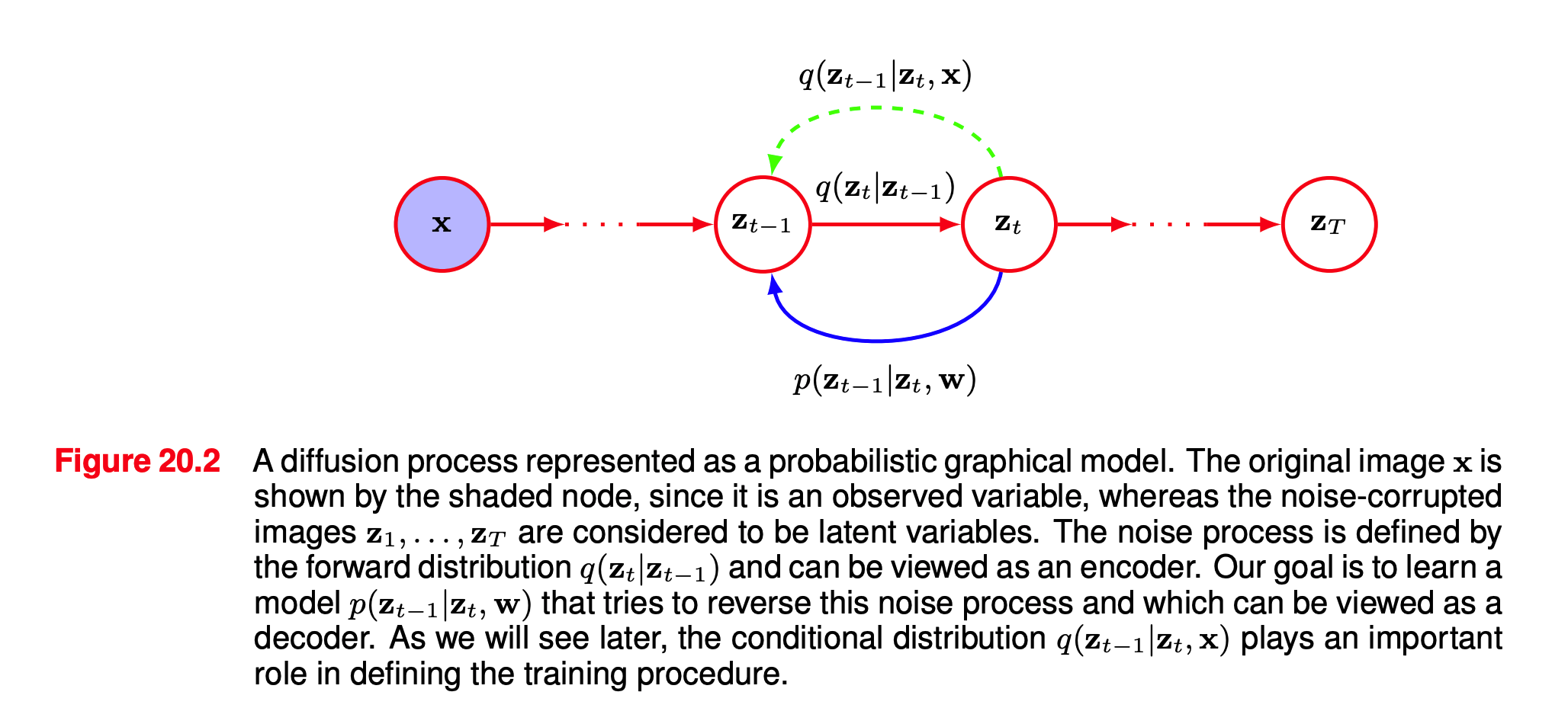
The Reverse Step We Want

The forward direction is easy because we chose it:

For generation, we need the opposite direction:

Bayes' theorem says

The problem is that this is not something we can compute directly. The terms and depend on the data distribution, which is exactly the thing we do not know.

Strümke and Langseth (2023), citing Feller (1949), point out that if the step size is infinitesimal, the reverse process has the same kind of distributional form as the forward process.

So we use that as motivation and approximate each reverse step with a Gaussian.

Instead of trying to compute

we learn a model for it:

The model is parameterized as

Here

is the mean predicted by a neural network. The variance is fixed to the same schedule.

Why The Reverse Step Is Gaussian

Now let's derive why this Gaussian shape makes sense.

Start with the reverse transition again:

By Bayes' theorem,

Take the log:

Inside this conditional distribution, is fixed, so can be absorbed into a constant:

Now define

Recall the forward kernel:

So its log-density is

Using :

Substitute that into the quadratic term. Anything that only depends on goes into the constant:

Now use the Taylor expansion of a real function around :

For our case, use

So

Apply the multivariate Taylor expansion around :

with

Combining the forward likelihood term and this Taylor approximation gives

Also,

When is tiny, is huge, so the leftover part is small compared with it.

So we approximate the log reverse transition as

Let

Now put back in:

Expand the quadratic:

Now keep only the terms that depend on :

A Gaussian log-density can be written as

Comparing coefficients, we get

which means

So the reverse transition is Gaussian-shaped, with variance and some mean.

We let a neural network learn that mean:

So the forward process is

and generation tries to run it backward:

When is small, this backward step can be approximated as

The variance is fixed, and the neural network learns the mean.

Evidence Lower Bound

The Learnable Reverse Trajectory

So far, the reverse transition is approximated by a Gaussian:

and the mean comes from a neural network:

The true reverse trajectory can be written like this:

We replace it with a learnable model:

where

Why We Need The ELBO

Ideally, we would choose by maximizing the likelihood of the data:

Equivalently, maximize

But this is hard to compute directly, because we would need to integrate over every possible trajectories:

Instead, we'll show that this likelihood has a tractable lower bound ELBO:

And if so, instead of maximizing directly, we can maximize the lower bound. As the lower bound goes it, it raises the likelihood up.

Let . The identity we want is

where

and

Because ,

So is the ELBO. But how do we get there?

Deriving The ELBO Identity

Start with

because .

Use

Then

Now multiply and divide by inside the log:

Then split the log:

So we get

Now here's the coolest thing!!! This works for any choice of , which means we can choose which is the forward diffusion process we already defined!

Let's do that substitution then we'll have:

The reverse generative model factors as

The forward process factors as

So

Expand the log:

Rearrange it:

The first term uses the fixed distribution . The third term also does not depend on . Since neither changes the trainable parameters, we can ignore them for optimization.

So for optimizing , the part we care about is

Now take expectation under the forward process :

By linearity of expectation:

One Transition Term

Now look at one transition term:

Define

Then

This is an integration over the whole trajectory , but it's quite conspicuous that there might be away to rewrite it to depend only on and . We'll do exactly that below.

Using the forward factorization,

Substitute the forward factorization:

The function only depends on and .

So variables after can be integrated out one by one:

and so on, until only terms up to remain.

Therefore,

Next, we integrate out the earlier variables .

Recall the marginalization identity

Applying this to the forward chain,

Then,

Repeating this up to , we get

Putting back in, one transition term becomes

Indeed, we've remove all other steps in the trajectory except for and . Let's continue.

The numerator is the learned reverse step:

The denominator is still the forward step:

But what we want is a comparison between

So let's reverse that !!! We have:

Therefore,

Substitute this into the log:

Split the log:

The first term contains the model. The second term does not depend on , so it becomes part of the constant.

Dropping the -independent parts, the transition term is

The inner part is the negative of a KL divergence:

So this transition contributes

Maximizing this is the same as minimizing

Now the ELBO can be written as

where

The first term is the consistency term. It makes the learned reverse transition match the true reverse transition.

The second term is the reconstruction term. It makes the last denoising step recover from .

For reconstruction, use

During training, sample , predict , and compute

The Consistency Term

Now focus on the consistency term.

Take one of them:

We already made Gaussian. Now we show that is also Gaussian and has a closed form. Then becomes KL between two Gaussians.

Use Bayes again:

By the Markov property,

so

The forward transition is

Also,

Since does not depend on , it is constant when we view this as a distribution over .

Therefore,

So is proportional to a product of Gaussian-looking terms. Expanding the exponent and collecting terms in gives

where

and

The learned reverse model is

So the consistency term is

KL Between Two Gaussians

Assume we have two Gaussians over the same variable :

The KL divergence is

Equivalently,

Recall the Gaussian log-density:

and

Substitute the two log-densities:

For learning , only this term depends on :

Therefore,

Now rewrite

Thus,

Expanding,

Take expectation under :

But

and

Therefore,

So

Matching Gaussian Means

When the variances are fixed, learning through Gaussian KL turns into matching the means:

So, up to constants and weights, this term is

To compute , sample and calculate the true posterior mean

The model gives its own reverse mean, .

So this loss compares

This already gives a valid objective. But there is a nicer way to parameterize it.

Predicting Noise Instead Of The Mean

Recall

Rearrange it to solve for :

The true posterior mean was

Substitute the expression for , use , and simplify:

The neural network is supposed to learn the reverse mean

But instead of asking it to predict the whole mean directly, we can build part of the structure into the formula.

Since the mean only depends on , , and , define

This is like keeping a fixed path through and only asking the network to predict .

In other words, instead of predicting the mean, the network predicts the noise.

The true posterior mean is

The model mean is

Subtracting them gives

The consistency term was

Plugging the difference above into it gives

So training the reverse process is really training a network to predict the noise .

The Reconstruction Term

Now we can fold the reconstruction term into the same idea.

Start with the reconstruction term:

At , the forward process is

Since

we get

Solve for :

Use the same noise-prediction form for the model mean:

Then

For , we had

For , , so

This is exactly the reconstruction term. So reconstruction is just the case of the same noise-prediction objective.

The Full Noise-Prediction Objective

So the whole objective can be written with

where

In this noising and denoising setup, training the diffusion model means maximizing the ELBO:

Equivalently, minimize the negative ELBO. After rewriting the consistency terms and the reconstruction term, the loss becomes

where

The Simplified DDPM Loss

In practice, DDPMs usually drop the time-dependent weight . The simplified loss is

Here we sample and , then directly construct

Then feed and into the neural network to get . The model learns to predict the exact noise that was added to .

Sampling

At inference time, start from Gaussian noise and denoise one step at a time:

Algoirthms (taken from Bishop's book).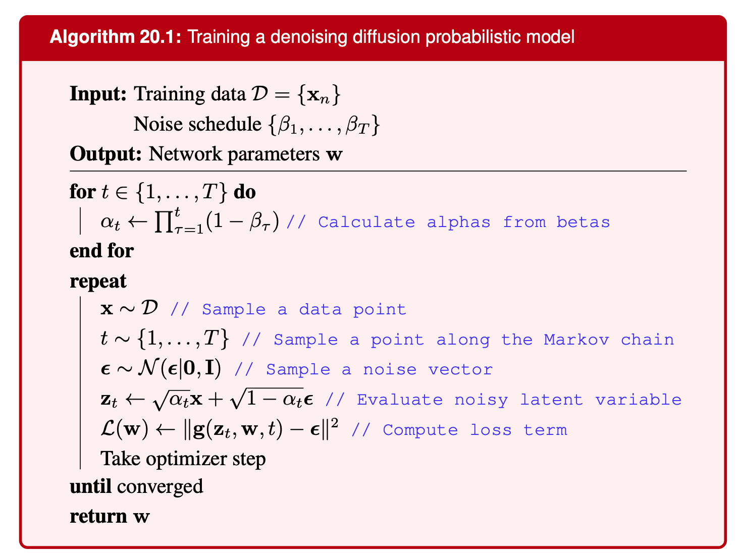

Code Example

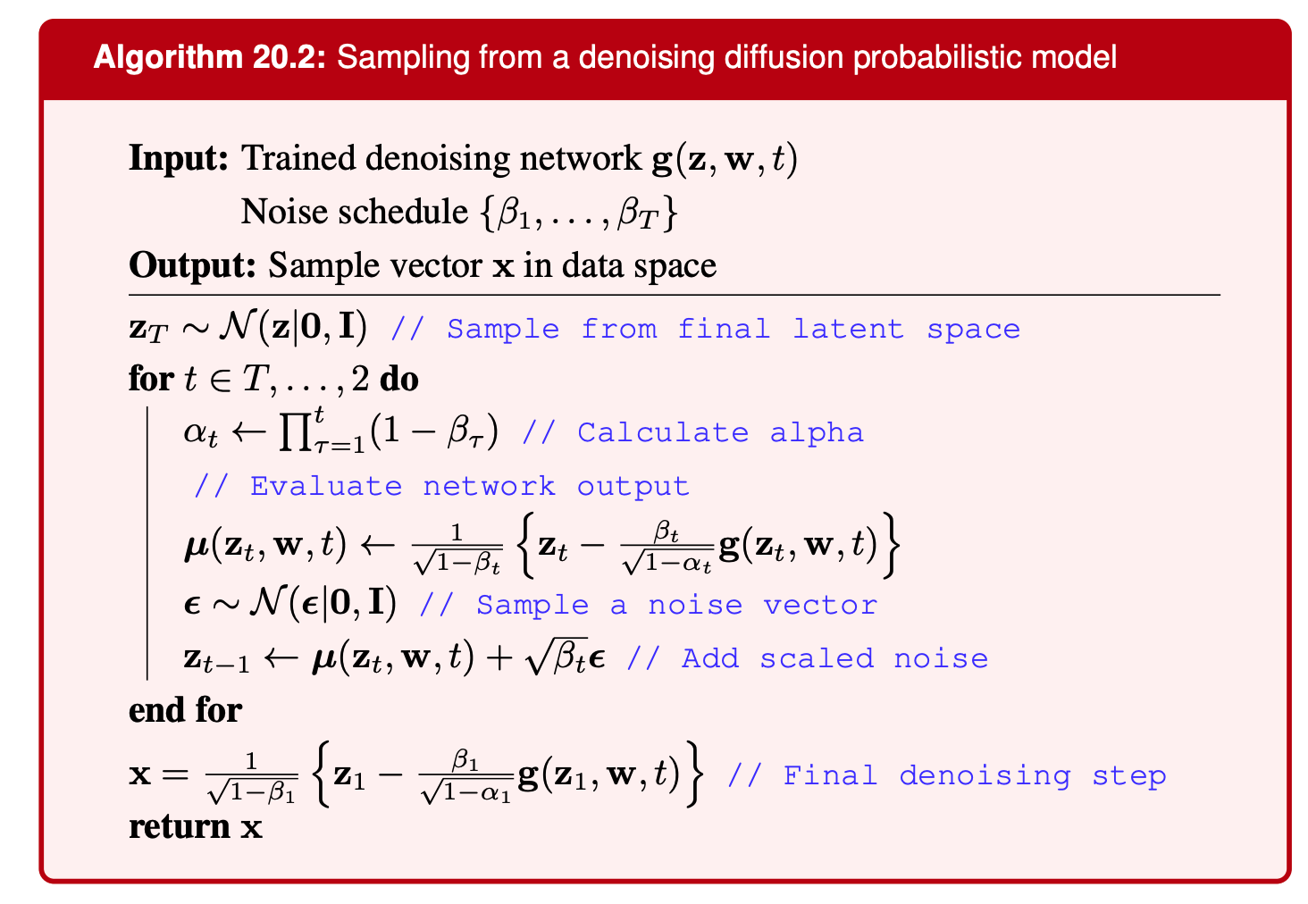
Once we understood the maths behind, we see that training a (simple) DDPM is very simple (duh?). I didn't write this code, instead I asked chatGPT to write it for me. It's a very small and simple model, trained with the original DDPM algorithm on MNIST data. I trained using the default settings for 100 epochs and got some interesting results.

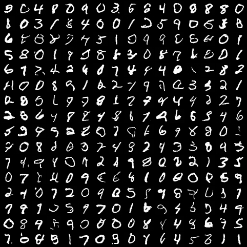
It's not the best, and I previously did get much better result training a larger model for a bit longer. But given I'm using my MBP with only 18GB RAM, it ran for 100 epochs at 22s/epoch and got this result, that's pretty sweet 🙃. You can find the code, the trained ckpt, and some generated samples in this repo. Finally, here are some animation of the denoising process from that model:

References

• Ho, J., Jain, A., & Abbeel, P. (2020). Denoising Diffusion Probabilistic Models. arXiv:2006.11239. https://arxiv.org/abs/2006.11239
• Feller, W. (1949). On the theory of stochastic processes, with particular reference to applications. In Proceedings of the First Berkeley Symposium on Mathematical Statistics and Probability, Vol. 1, pp. 403-433. University of California Press.
• Bishop, C. M., & Bishop, H. (2023). Deep Learning: Foundations and Concepts. Springer Nature.
• Strümke, I., & Langseth, H. (2023). Lecture Notes in Probabilistic Diffusion Models. arXiv:2312.10393.